10 Road Systems
Field reconnaissance work was held a little longer than the originally scheduled three-week period. We began our field work on Thursday April 27, 2003 and ended on Tuesday May 20, 2003. However, we were not in the field every day of the week as we took office days every Friday and also sometimes during the week. During this three-and a half-week period, the weather varied from sunny to rain showers to hail to snow. In fact, we even encountered heavy amounts of snow pack when setting grade lines at altitudes higher than 4000 ft.
The North Tahoma Forest landscape was predominately surrounded by private landowners on both sides of our boundary line with the Nisqually River bordering the north and State Highway 7 bordering on the south. Once all our preliminary pegging and road design process was finished, as well as our prioritization, we were ready to head out and start grade lining some of the roads we had proposed in the office.
Before entering our field reconnaissance phase we needed to prioritize our work in the forest due to time constraints. As a result, only those roads with utmost priority were field verified. The main criteria used for prioritization was the following:
- Mainline Systems
- DNR Laid Out Timber Sales
- Orphaned or Abandoned Road That Can be Activated as a Mainline
- Terrain and Weather Conditions
10.2.1 Planned Mainlines
During the four weeks of preliminary office work, mainlines were designed to access large areas within the project area. These roads were given top priority during the field reconnaissance since the road network hinged on the feasibility of these roads.
10.2.2 DNR Laid Out Timber Sales
Before our project had even started the DNR had already laid out three timber sales within our project area. Knowing these sales would be up for bid in the near future, it was also critical to make sure these sale units had the appropriate landings and roads connecting them to a mainline network.
10.2.3 Orphaned or Abandoned Road That Can be Activated as a Mainline
Currently there are old railroad and truck grades throughout our project area. These roads were used for logging most probably around the 1930's. Some of those grades are located well, however, they do not comply with present standards of maintenance and some have also suffered from landslides and erosion. In a few occasions, such grades were being used provided they were in the right location in relation to terrain features and current harvest system requirements.
10.2.4 Terrain and Weather Conditions
Sometimes our field work was governed by the present terrain and the weather conditions. Some areas within our project, particularly those above 4000 feet, were covered by pretty heavy snow packs yet this did not impede us from setting grade lines in many of these areas. On the other hand, roads which we had planned in the office were really not feasible in the field. In particular there was such an area in the Ridge Mainline system (Lake Creek). We walked a road we proposed on paper but determined there was too much slope instability to proceed. In the end, we decided helicopter logging would be the only real solution in gaining access to these areas in the Lake Creek area and their respective timber.
10.3.1 Setting Grade lines
The first step in our field reconnaissance process was to take our original pegged designs and set grade lines out in the field. This step was done using orange flagging, making sure we marked our flagging for the distance traveled in station numbers and the grade used. To guide us in the field, GIS maps were plotted with our pegged road lines. Once in the field, clinometers were used in order to guide our grade across the mountainside. This portion of filed reconnaissance work helped us identify problems, better options and the viability of what we had planned in the office out in the field. Careful note taking was done for every grade line set. Reconnaissance reports for each field day can be found in the appendix section of this report.
10.3.2 Setting and Brushing P lines
The next step after grade lining a road and being pretty certain that it will work is to set and brush a P line. P line simply refers to where the very center of our road will probably be. Depending on the road width, the P line will almost be anywhere from 5 to 15 ft. above up slope from the grade line. Our main concern with the P line is its adjustment and alignment. One must make sure to straighten out our portion of roads as much as possible during this stage of field work. Unlike the orange flagging used when grade lining our road, wooden stakes and blue flagging was used for our P line. In addition to proper alignment we also had to make sure we had good visibility of our points, meaning a person standing at a stake should have a clear line of sight to the previous and proceeding stake. This process often involved cutting out twigs and branches that impeded us from seeing stakes. Due to time constraints the Closer Mainline was the only road we brushed a P line for.
10.3.3 Traversing and Blazing
Once our P line stakes and lines of sights were established, our next step was to traverse and blaze our line. A criterion was used to traverse our line but we ran into some problems during its use. Slope distances and percentages were gathered from the criterion but a staff compass was used to gather compass bearings since the criterion compass was always off by three to five degrees. GPS points as well as traverse loops were used in order to close our traverses and get our precision. Also being careful to take good notes in the filed helped us determine our precision which came out to be 1 in 715. A staple gun and flashers were used to assign point numbers to our stakes. Distances between stakes fell below a full station and were spaced on average about 70ft. In addition to the steps mentioned above we also had to make sure our line and points were clearly visible for anyone entering the forest. To do this, we used orange spray paint to "tag" our stakes as well as several trees along our line.
10.3.4 Stream Survey
As a part of the "Closer Road" traverse, we preformed a stream site survey on the first stream crossing. Our preliminary analysis concluded that we should use a portable bridge at this location. The stream survey was the next step in finding the best solution for this crossing.
The survey was conducted on May 20, 2003. The crew consisted of Mark, Colin, and Jeremy. The weather was overcast with light rain towards the end of the day. The MapStar Laser was used to collect and record the data for our survey. Jeremy ran the MapStar, while Mark and Colin occupied the appropriate points with a staff and reflector prism. Due to light brush conditions only two points needed to be occupied by the laser.
The survey we conducted was a two part process. The first part was a terrain survey, *-and the second part was a Thalwag survey. These two were combined to give us an accurate model of the stream.The first survey we did was the terrain survey. The purpose of this was to capture the important terrain features of the stream channel. To do this we ran nine cross-sections perpendicular to the stream channel. These cross-sections went one and a half stations up and down the stream and extended 50 to 75 feet on both sides of the stream channel. The points that were taken identified critical terrain features, hig water marks, the wetted edges of the stream, and the thalwag of the stream. The cross-sections were taken at points along the stream that would best identify changes in the stream channel.
The Thalwag survey consisted of several points taken along the centerline of the stream. These points were carefully selected to capture the direction and grade of the stream channel. This survey went approximately 2 stations up and down the stream. Overall, 129 points were recorded in both surveys.
While we were there we also did some recon upstream of the crossing location. We found fish blockages approximately 3 stations upstream of our crossing location. The side slopes were steep and unstable, large boulders and debris are being deposited into stream from side slopes. This gave us a good understanding of what kind of material would have to be able to pass underneath the bridge.
Once the Closer Road was traversed, the data obtained in the survey was entered into RoadEng and a design was produced. Overall, 116 + 86 stations were designed. The design that was produced included a profile, a plan view, and cross-sections.
For our design three different road templates were used. For these templates the road width was 12 feet and the rock depth was 12 inches. The cut slopes were calculated to be 1 to 1 and the fill slopes were calculated to be 1.5 to 1. The ditches that were used were given a width of 3 feet and a depth of 1 foot. The road surfaces were crowned and outsloped at -3 %.
The first template was used for the first 4 + 37 stations, and it had a ditch on both sides of the road. This section of road was a large through cut for the first switchback. Two ditches were used in this location to keep water off of the road surface.
The second template was used from stations 4 + 37 to 58 + 67, 63 + 77 to 100 + 00, and 102 + 89 to 116 + 86. This section of the road had steep side-slopes that dropped off to the left. For this reason the template that was used had a ditch on the right side and a crowned road surface. Much of this road had to be full bench because the side-slopes exceeded 45 %.
The final template that was used was outsloped to the right. It was used on stations 58 + 67 to 63 + 77, and 100 + 00 to 102 + 89. This template was chosen for these areas because the side-slopes were pretty mild, and a ditch would not be necessary.
There were three stream crossings on this road. The first stream crossing is the largest, and will most likely be crossed with a bridge. For our preliminary design we estimated that the other two stream crossings would have a 6 foot pipe. There were 31 crossdrains on the road.
The following section describes each road system present in our project area. Even though our field reconnaissance time did not allow us to set grade lines in every road system we designed, descriptions for this roads were also made and can be found in the following sections.
10.5.1 Closer System
The Closer Mainline road system consists of one major road with several spurs, which access landings within the Closer and Schwing Ding timber sales. This road is located in the northwestern part of the planning area covering approximately 341 acres and spanning for 117 stations (2.2 miles).
The Closer Road spurs off the #10 road in the SW � of the SW � of Section 33 of T15N R06E. The road continues in a northwesterly direction until reaching the outer boundaries of the Closer timber sale. The road consists of three switchbacks. The first one is situated at the point from which it starts off from the #10 road and the other two are both located in saddles between ridges.
There are two major stream crossings which determine the location of this road. It was determined that the original stream crossing location at the first stream was too low, which later placed the road in wet, unstable slopes leading up to the second stream crossing. To avoid these potential problems, the initial stream crossing was placed upslope past the confluence of the stream creating yet another crossing. However, this placed the road on stable slopes for this portion of the road.
The RoadEng design files can be found on the data CD
\final_dnr_data\mark\Closer Mainline RoadEng Design
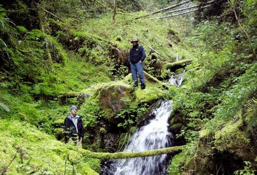
Figure 19: Mark and Colin stand near a fish blockage on the first stream crossed by the closer
road. This blockage was approximately 400 feet up stream from the proposed road crossing.
It was determined that since the first stream crossing has deeply incised channels, that a bridge would the best solution in crossing. In addition, the DNR also has a portable bridge not currently being used. A detailed stream survey was done at this site in which a 3-D image of the stream was generated and then traversed.
From the second stream crossing on (station 40+22), the road runs pretty smoothly, not crossing any potentially unstable areas. It runs down this ridge on the other side of the second stream crossing until it reaches a saddle on which we have our second switchback. From this switchback, 58+16, the road stretches out in a northeastern direction until it hits one of our landings at station 67+30. From this landing location, on which there are remnants of old truck or railroad grades, the road continues along the landscape in a northern direction and then curves around the northeastern ridge of the Closer sale to come back into the flat, saddle area near which our second switchback occurred. From this switchback (station 100+98) the road climbs up the northwestern ridge of the closer sale until it reaches a landing on the northern facing slope of the eastern half of the closer sale (station 116+86, GPS verified).
As mentioned earlier, there are several spur roads contained within the closer system. Although these were never verified in the field they consist of relatively short distances and should be pretty inexpensive to construct when the sale is ready for harvest. The first spur runs about 5+13 stations northwest from the main road. The spur begins about 14+50 stations from the first stream crossing. The next spur road starts of in between our second stream crossing and our second switch back, about 8 stations north from the stream crossings and runs east for about eight stations. We find two more spur roads taking off from our landing location at station 67+30, one running north for about 5 stations and the other running west for about six stations in order to access another landing. Two more spurs take off in a western direction for about four and a half stations each starting at station 82+55. The last and final set of spurs stretch out south for about nine stations starting out at about seven and a half stations from our last switch back. Figure 20 shows the entire Closer road system shown in blue.
Figure 20: Closer road system in blue. The settings in orange will be using the Closer road system.
10.5.2 Mineral System
The Mineral Mainline System consists of two major stretches of road and a system of spurs. There are two major purposes for this road system. The first is to access the southwest part of the North Tahoma block, and the second is to connect the 24 Road with the existing Mineral Road system (Figure 21). This road system accesses over 900 acres of harvestable timber with approximately 550 stations of new construction.
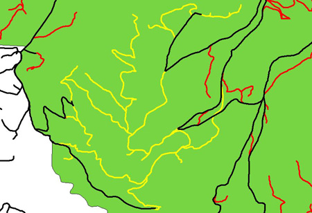
Figure 21: The yellow roads represent the Mineral road system.
The topography and slope stability of this area controlled the location of most of the proposed construction. There are several wet and unstable areas which we tried to avoid. We tried to stay away from these areas, because there are high maintenance fees of having roads in that area. Much of the road goes through steep side-slopes, which will make for high road construction costs due to the large volume of excavation.
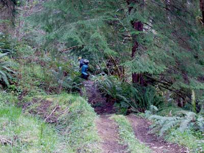
Figure 22: The lower existing Mineral road. After field verification
it was determined that this road should no longer be used.
Two different routes were looked at to connect the 24 Road with the existing Mineral Road system (Figure 23). This was done so that were could compare and contrast two different options and chose the best one. Both of these roads took advantage of old railroad grades (Figure 24). Some maintenance will have to be done on these grades to stabilize the slopes.
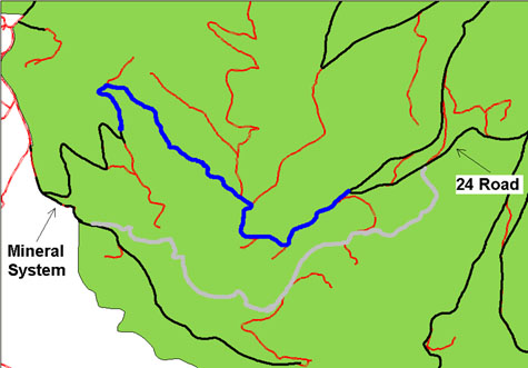
Figure 23: Upper (Blue) and Lower (Grey) Options for Proposed Mineral Mainline.
The first option that we looked at started approximately half a mile up the 24 Road and extended west to connect with the existing railroad grade in the Mineral system. There were multiple unstable areas (Figure 22) and difficult crossings (Figure 25) along this route.
Evidence of mass wasting and washouts were found along the length of the lower existing railroad grade (as seen on Figure 24), making its extensive use uneconomical. Several wet areas with alder trees and other water loving plants and were also found along the proposed route, indicating potential for future failure.
There were also two difficult stream crossings on this route with steeply incised channels (one is shown in Figure 25). These crossings would not require bridges, but the alignment must be pushed into the hill to reduce the fill height over the stream. This will result in large cuts.
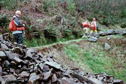
Figure 24: Failure on Old Railroad Grade.
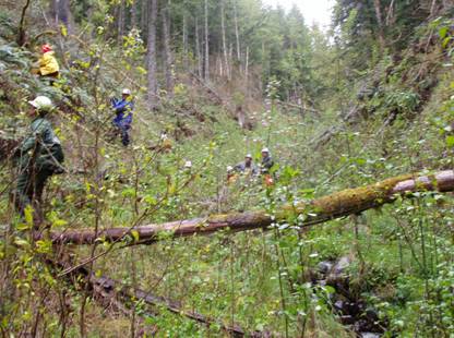
Figure 25: Difficult Stream Crossing.
The second option that we looked at started at the first switchback of the 24 Road and extended west, above the first option, to connect with the cork screw road of the Mineral system (Figure 23). The idea was to locate the route above the streams and wet areas that were in the lower part of the ridge.
There are a few engineering challenges in building this road. There were still several wet areas, with lots of alder that had to be crossed (Figure 26). Some of these locations were able to be avoided by moving the road up above the start of the wet area.
For 8+50 stations the road follows an existing railroad grade. There are two spots along this grade which have begun to become unstable due to a lack of water control (Figure 27). These two spots are characterized by deep stream channels. With careful road placement and appropriate culvert placement, these points can be crossed.
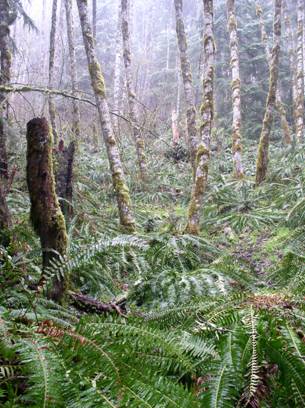
Figure 26: Potentially Unstable Area.
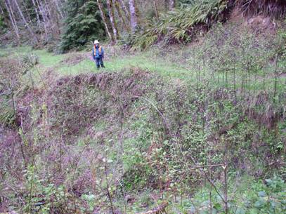
Figure 27: Failure of Old Railroad Grade.
In conclusion, both of the proposed routes connecting the Mineral system with the 24 road are difficult to construct and would require extensive maintenance following construction. Network analysis is needed to determine if savings in haul cost from routing trucks through the Mineral system (bypassing Ashford) will offset the significant road construction costs in this area.
10.5.3 West Mineral System
The West Mineral Road System consists of a one bypass as well as a few designed access roads (about one mile in length) combined with a system of spurs (Figure 28, in yellow). The major purpose for this road system is to access over 1,700 acres of harvestable timber with approximately 630 stations of new construction. The bypass route allows for two options for exiting the area, via the east wing or west wing.
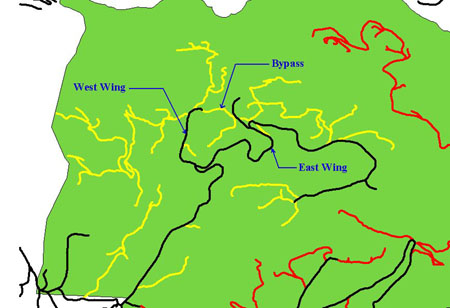
Figure 28: West Mineral Road System (Yellow).
The long designed access roads are necessary due to the limited extent of existing roads in this system (only 350 stations). Grade line was set in the field for the majority of these access routes. Limited grade line was set for spurs.
The bypass allows for trucks to exit on the west wing or the east wing of the existing portion of the West Mineral Road System. This will allow for Network calculations to find the haul route of least cost and sedimentation calculations to find the route of least sediment delivery.
No significant slope failures or hazardous areas for road construction were found in the West Mineral Road System. Due to the large extent of coverage in field work, no extensive slope failures are anticipated in other portions of the system. Existing railroad grades were used frequently due to good stability.
10.5.4 Ridge System
The ridge road system consists of one major road (the ridge road itself) and various spurs. This system access's the southern to southeastern areas of the North Tahoma block and it allows access into upwards of 1,893 acres and 82 settings. There are 469 stations of existing roads and 748 stations of planned roads within this system. With all roads combined totaling approximately 23 miles of roads within the system (Figure 29).
While the road primarily accesses the northern slope of the ridge it is located on the southern side due to the steep slopes and visual issues, caused by the close proximity to highway 706. There are two main spurs branching off the ridge road, one accessing more of the North Slope, and the other accessing the southwestern slopes of the ridge.
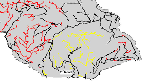
Figure 29: Location of the Ridge system leaving the 23 Road. The yellow roads are the ridge system.
The Ridge Road splits from the 23 Road in the NE ¼ of the SE ¼ of Section 9 of T14N R06E. The road continues in a northerly direction, and then curves to the west, from a saddle and continues along the ridge. The road ends when it reaches the nose of the ridge where the western most landing on the ridge is planned. The southwestern spur was originally planned to come off the existing spur just after it left the 23 road, but due to some stability issue it was broke into two separate spurs to access the necessary landings. The spur that accesses the rest of the North Slope leaves the ridge road at approximately station 37+00 and bears due west. The haul routes out of the ridge system and its spurs will, for the most part, be an adverse haul due to the high elevation of the spur coming off of the 23 road. Since there was no other way to access this area the adverse haul could not be avoided.
The Ridge road mainline never crosses any streams or wet areas thus stability is not an issue for the mainline. However the spur that accesses the southern to southeastern part of the region has some stability issues. Most of these stability issues were avoided by breaking the single spur into two different segments avoiding the unstable area. The other main spur was not field verified due to time constraints. There are various other short spurs leaving the ridge road that were not field verified. These are mainly short spurs that should be fairly inexpensive to construct.
The Ridge system is the largest road system within the North Tahoma planning area and accesses the largest acreage of all of the systems. Due to time constraints we were only able to field verify the mainline and one of the main spurs. So there is some extensive field work to be done in this area. Do to visual impacts and the steepness of the terrain some of the spurs in this area may have to be moved and or some adjustments made during the field verification.
10.5.5 Reese Creek System
The Reese Creek Road System consists of one major cutoff road and a system of spurs. There are two major purposes for this road system (Figure 30). The first is to provide a cutoff for the 24 road, eliminating 2 stream crossings and approximately 62 stations of parallel roads. The second purpose of this road system is to access 570 acres of harvestable timber with approximately 134 stations of new construction.
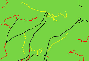
Figure 30: Reese Road System (Yellow).
With so few new stations, the Reese Creek is a small road system. However, the cutoff would help reduce haul time down the 24 road. Most of the area is harvested with a mobile tower and can be accessed with existing roads. The few planned spurs help reach landings for primarily central tower settings as well as a few ground based and mobile tower settings.
Only a minority of the grades in this area were ran in the field since there was only one proposed change to the main haul route. The 24 cutoff was set with no major difficulties. A minor area of concern is the initial routing off the 24 road, which is adjacent to a stream buffer. The area here is steep and construction will be difficult next to the wet areas of the buffer.
The next grade line set in the field was an alternate route accessing the southern landing of the Schwing B sale. This spur runs to the south of the proposed route, increasing the spread between the spurs for this area in about the same length of construction.
No significant slope failures or hazardous areas for road construction were found in this area. However, as mentioned, field work was limited in the Reese Creek Road System, so problem areas may exist.
10.5.6 Catt Creek System
The Catt Mainline road system is the smallest road system of our road network. It consists mainly of several small spurs that extend off of the existing road network. These roads are located in the southeastern part of the planning area, covering approximately 439 acres (Figure 31).
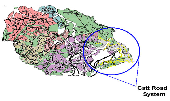
Figure 31: Catt Road System.
The Catt system consists of 587 stations of roads (Figure 32). There are 108 stations of new roads that we have planed for that area. Due to the time constraints of the quarter, the only road in this system that had field verified was the last 15 stations of the "Ridge road." There were no stream crossings on any of the new roads that were laid out.
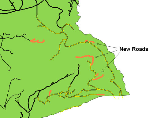
Figure 32: New Roads on Catt System.
After completing the field reconnaissance part of the design process we were able to analyze grades, side slopes, stream crossings, and unstable areas using the field data and our planned roads. Below is a map that illustrates the status of the roads within the study area. Black represents the existing roads, red represents the roads where the gradeline has been laid out in the field, and the blue represents the planned roads within the study area (Figure 33).

Figure 33: Map of the Road Status within the North Tahoma Planning area.
Using ArcView within GIS we were able to come up with some length statistics for the different road status. Below is a table that illustrates the various station lengths for the different road status categories.
| Gradelined | Traversed | Planned | Existing | |
| Stations | 1099 | 117 | 1163 | 2811 |
Road lengths/Streams
When designing roads our goal was to limit the number of stream crossings and the amount of road adjacent to streams. Of course we did have to cross some streams to access the necessary timber. Below is a table that represents the total length of existing road and planned road. It also shows the number of stream crossings and the number of stations within 200 feet for each road status and the total. The last column in the table shows the number of stream crossings per mile of road for the Existing roads, UW designed roads, and the total road system within the North Tahoma planning area.
| Road Status | Total Stations | Stream Crossings | Stations (Within 200 ft. of streams) | Stream Xings/Mile of Road |
| Existing | 2811 | 75 | 1047 | 1.41 |
| UW designed | 2379 | 49 | 793 | 1.09 |
| Total | 5190 | 124 | 1840 | 1.26 |
Grade Distribution for UW roads
During the design process of our road system where ever possible we strived to stay under a maximum grade of 18%. We achieved this both in the office and in the field and the table below represents the grade breakdowns on the roads that are planned and gradelined. I did not perform a grade breakdown on the existing roads due to the inconsisticies in the Trans layer between road locations and DEM we received from the DNR. The road segments were too long giving an inaccurate depiction on how the grade changed from point to point. So to analyze these road segments would have been pointless.

Figure 34: Grade distribution for all UW roads.
Side Slope Breakdown on all UW and Existing roads
We were not able to field verify all of the roads in our study area due to time constraints, but we were able to analysis on sideslopes on all of the roads. We did this by manipulating the attribute tables within GIS to achieve a sideslope output on all road segments including all existing and UW designed roads.

Figure 35: Sideslope Breakdowns on all roads in the Planning area.
The data reflect the fact that new road systems have to access more difficult terrain not yet reached by the existing roads. As a result more of the roads are on steeper sideslopes.
Mainline access systems
Within the North Tahoma planning area we separated our road system into six different mainline systems. These systems are the: Catt, Closer, Reese, Ridge Mineral, and West Mineral mainline systems. These systems access a total of 5,900 acres of timber within the North Tahoma. Below you will see a map illustrating the different locations of the mainline systems throughout the North Tahoma planning block. The different systems are color coordinated and those colors show up in the key.

Figure 36: Map illustrating the locations of all six mainline systems (Yellow=Catt System,
Blue=Closer System, Red=Reese System, Pink=Ridge System, Light Blue=Mineral System,
Green=West Mineral System).
After the six mainlines were established in the North Tahoma we were then able to run some individual statistics on each system within ArcView. Below is a table that illustrates some of those statistics. Table 12 does give the planned and existing road data for the individual systems and the acreage and settings accessed within those systems.
| Road System | Catt | Closer | Mineral | Reese | Ridge | West Mineral |
| Planned (Stations) | 92 | 199 | 550 | 134 | 748 | 631 |
| Existing (Stations) | 396 | 2 | 171 | 261 | 469 | 353 |
| Total (Stations) | 488 | 202 | 721 | 395 | 1217 | 984 |
| Area (Acres) | 493 | 341 | 910 | 568 | 1893 | 1747 |
| Number of Settings | 21 | 20 | 43 | 27 | 82 | 70 |
10.7.1 Road Construction Cost Estimates
A preliminary cost analysis was performed to determine road construction expenses. Each road option that was "pegged in."
In order to develop an estimate, the "North Tahoma Road Costing" spreadsheet was developed. This tool was created using several different sources of information. These included old cost analysis spreadsheets used by past classes, reports that were developed specifically for cost analysis, as well as information gathered by talking to a rock quarry manager. The information that was gathered included production rates, as well as formulas that were used to calculate variable areas and volumes of road construction. We used several different sources of information.

Figure 37: Road Costing Spreadsheet.
The original layout of the spreadsheet followed the same format that was used by past classes (see Figure 37). Unique variables such as length, side-slopes, road-width, and haul distances were entered into the spreadsheet and a total cost, and a cost per station were produced. About 20 variables were used in the spreadsheet.
All of the variable costs and production factors that were used in our spreadsheet were put into the "Cost breakdown page" (Figure 38). The spreadsheet was designed so that by changing any variable on this page, would also change every location of that variable on the main page. This allows the spreadsheet to be quickly updated. As with any costing analysis, the better the input data, the better results you will receive. In this case, local rates for particular contractors should be inserted where appropriate.

Figure 38: Cost Breakdown Page.
Unlike past year's projects, we did a cost analysis for every individual segment of pegged road (Figure 39). This gave us a cost estimate, for every road option, early on in our design process. Originally, we tried to use the spreadsheet to analyze each individual segment of road. This did not work because there were thousands of segments to look at, and there was no easy way to automate the process through Excel. To compensate for this problem we used the power of G.I.S.

Figure 39: Example Road Segment.
Using our spreadsheet, we developed a table (Figure 40) that gave prices for road construction based on side-slopes and the distance to the closest rock pit. For side-slopes ranging from 0 to 90 percent and rock haul distances from 0.5 to 10 miles, prices were given for excavation, pioneering, right-of-way logging, clearing, grubbing, grading, compacting, ditching, culverts, and ballast. These prices were given with the assumptions that the average MBF per acre was 33 (This number was determined from the silvicultural data for our area.), the maximum distance for end-haul was 1 mile, the road width was 10 feet and 9 inches of ballast was placed on each road. After this table was created, it was exported into G.I.S.

Figure 40: Road Construction Side Slopes.
Phil Hurvitz wrote several A.M.L.s, inside of G.I.S. which automated the cost analysis process. The first step in this procedure was to add data fields to each segment of road. The fields that were added were line-slope, side-slope, length, road name, cost and grade (Figure 41). The first three fields were calculated by referencing each line segment to the lidar digital elevation model. The name field was manually entered, and the grade field was filled by referencing the grades that were used during the actual pegging of the roads.
After these fields were added and filled the cost field was then calculated. This was done by taking each road segment and determining the distance to the closest rock pit and then referencing it to the cost analysis table. Based on the side-slope and the rock haul distance, a cost per station was looked up. This cost per station was then multiplied by the length of the segment to determine its cost.

Figure 41: Road Attribute Table in GIS.
Once the cost field was filled we could easily select any group of roads from our network, and quickly determine the price of that segment.
10.7.2 Variables Analyzed for Costing
Move in Costs
This section was added to estimate the cost associated with moving a piece of equipment to the construction site. This section allows you to choose the number of each equipment you will have working on the road construction.
Pioneering
Costs for pioneering of a road can be calculated for using either a crawler tractor or an excavator. These prices are based upon a station per hour basis. The information for this section came from John Balcom's, "Construction Costs for Forest Roads."
Right-of-Way Logging
Right-of-way logging can be done either by tractor or excavator. The cost that is developed is determined by MBF per acre, as well as the clearing and grubbing limit that is chosen in the next section. The average MBF per acre for our working area was 30.
Clearing and Grubbing
This section will give a cost for clearing and grubbing based upon MBF per acre, the clearing and grubbing width, and the number of stations being built. It also will generate different costs based on the side-slopes of the area. There is a cost that can be developed for an excavator as well as a tractor. These costs are assuming that the clearing and grubbing is being completed at the same time as road construction.
Excavation and Embankment
Since there are so many variables in this part of road construction, this is one of the most detailed parts of the spreadsheet. Prices can be developed for the use of a tractor, an excavator, or a scraper on either easy, medium, or difficult side-slopes. This section is based upon a cost per cubic yard of excavated material. This volume of excavated material is calculated by a given side-slope, cut slope, sub grade and ditch width, and total number of stations. These numbers can all be entered in manually, which can greatly increase the excavation volume estimate.
There is also a section to deal with the mass haul associated with road construction. The variables for this section include bucket capacity, cycle time, operating efficiency, distance to waste site, truck capacity, and truck speed. The price of end-haul will also be adjusted with the number of dump trucks that are selected.
Sub-grade Finishing
This section provides the least detailed cost analysis. The number that was used, $60 per station for grading, compacting, and ditching, was found in "Construction Costs for Forest Roads."
Installing Culverts
By inputting the number of culverts needed by diameter, this section will compute the cost to purchase and install the needed culverts. The prices were obtained from Washington Culvert Company. The important thing to note here is that the break-even point, based on purchase price alone, between plastic and metal pipes is at 24 in. diameter. Below that, purchase plastic, above that purchase metal. For analyzing the cost of pegged segments, the price of $100 per station was used for culverts.
Surfacing
This section allows you to calculate the amount of rock that will be placed on the road, based on thickness of rock, width of road, and length of road. Sections of different road widths and thicknesses can be entered at the same time. There is a price that is developed for hauling that volume of rock. Calculations similar to the end-haul analysis were used. Since rock for the roads will be obtained from nearby rock pits, the entire expense of the rock is based upon the haul distance.
Erosion Control
Prices for applying seeding, fertilizing, and hay mulch, are calculated in this section. The area of cover is determined from the length of road and the fill and cut slope cross-section. These cross-sections are pre-calculated, based upon the width of the road.
Overhead
Overhead for this project is assumed to be 10%, but this can be manually changed if desired.